How NucleusAI Curated a 1.5B Image Dataset for Generative Vision Models
2026-02-03
Building an image model is only partly a modeling problem. The other part is a data engineering problem disguised as a plumbing problem, which is a polite way of saying: "if your dataset is messy, your model becomes an expensive mirror for that mess."
NucleusAI built an end-to-end pipeline to curate an image dataset with quality controls that treat data like a first-class product, not a folder of “stuff.”
This article covers The Dataset: collection, validation, cleaning, scoring, captioning, and packaging.
The Core Principle: Scale is easy, signal is hard
“More data” is a trap phrase. You can always collect more. What matters is:
- Validity: can you decode it, trust it, and locate it again?
- Alignment: does the caption describe the image accurately?
- Quality: is it useful for the model you’re training, not just “a JPEG”?
- Control: can you shape the distribution (curriculum, tail sets, domain mixes)?
Everything below is us building that control plane.
Phase 1 - Metadata Backbone: A Billion-Row Truth Table
We never relied on a centralized database to track our metadata. From day one, the architecture was designed to be schema-controlled, cloud-native, and columnar. Every record existed in partitioned Parquet files, with 50,000 rows per file. This format gave us faster sequential reads, predictable sizes, and excellent compatibility with the rest of our pipeline (sampling, training, and analytics).
Each Parquet file was:
- Aligned to a deterministic shard index
- Compression and Encryption enabled (when staged to cloud)
Schema (training-facing)
Key choices within the training schema shape we converged:
idserved as the stable primary key across the training corpus.source_idprovided lossless traceability back to the upstream record.captions[]are ordered from lowest → highest quality, and if an “internet caption” existed, it stayed at the top so we never lose provenance.caption_sources[]is a one-to-one mapping of thecaption_sources[i]to thecaption[i].partition_keyis a uniform integer used for deterministic sharding and mixing.
Why Parquet
- Columnar format: Columnar storage avoided deserializing entire records. All our downstream experimentation and training jobs often only needed specific fields.
- Splittable for compute: We laid out the Parquet files so that row groups became our scheduling unit, then we sharded the work so each worker processed a disjoint set of row groups with no read amplification. This kept ingestion tight under parallelism. Workers only read what they were responsible for, so throughput stayed predictable.
- Storage-aware: We leaned on column pruning + compression so object-store reads pulled fewer bytes and decompressed only the columns we trained on. That reduced load time and cost while keeping performance stable as the dataset scaled.
How we wrote and operated on it
We wrote metadata using PyArrow writers in streaming mode, with validation hooks to ensure schema consistency across files. All processing (ETL workers, captioning workers, samplers) used Pandas + PyArrow to interact with the metadata.
import pyarrow as pa
import pyarrow.parquet as pq

schema = pa.schema([
	("id", pa.string()),
	("source_id", pa.string()),
	("captions", pa.list_(pa.string())),        # captions[] preserves order
	("caption_sources", pa.list_(pa.string()))  # caption_sources[] map 1:1 to the above list
])

with pq.ParquetWriter("metadata.parquet", schema=schema) as writer:
	for batch in stream_batches():
        table = pa.Table.from_pylist(batch, schema=schema)
        assert table.schema == schema
        writer.write_table(table, row_group_size=25_000)
This choice of moving away from classic databases was fundamental to maintaining throughput at scale. Instead of overloading Postgres or BigQuery with billions of rows of rapidly changing state, we opted for a declarative, columnar log for the dataset metadata.
This gave us fast filtering and joins, repeatable slicing and lightweight shuffling and sampling (since all files had the same row count and fields)
To this day, our entire dataset pipeline treats Metadata Parquets as the source of truth.
Kafka as the Orchestration Spine
Kafka sat between “metadata exists” and “pixels exist.” That boundary mattered as the pipeline became distributed, retryable, and observable.
Producers streamed metadata records into Kafka topics; Consumers handled download → validate → persist. We used Go clients (Sarama and kafka-go) depending on the worker’s needs (simple fan-out vs. richer group semantics and control)
At a high-level, we kept the working logic simple.
// Download Consumer
for {
	m := fetchMessage(ctx)
	id := string(m.Key)
	if alreadyProcessed(id) {
		commit(m)
		continue
	}

	var err error
	for attempt := 1; attempt <= maxAttempts; attempt++ {
		err = downloadValidatePersist(id, m.Value)
		if err == nil {
			markProcessed(id)
			commit(m)
			break
		}

		if attempt < maxAttempts {
			time.Sleep(baseBackoff * time.Duration(1<<uint(attempt-1)))
		}
	}

	if err != nil {
		publishDLQ(id, m, err)
		commit(m) // commit after terminal handling to avoid hot-looping
	}
}
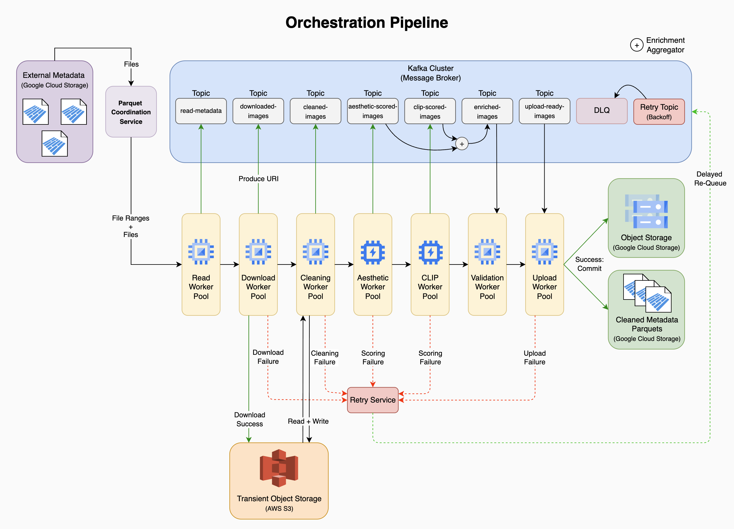
A full end-to-end orchestration diagram is shown in the appendix.
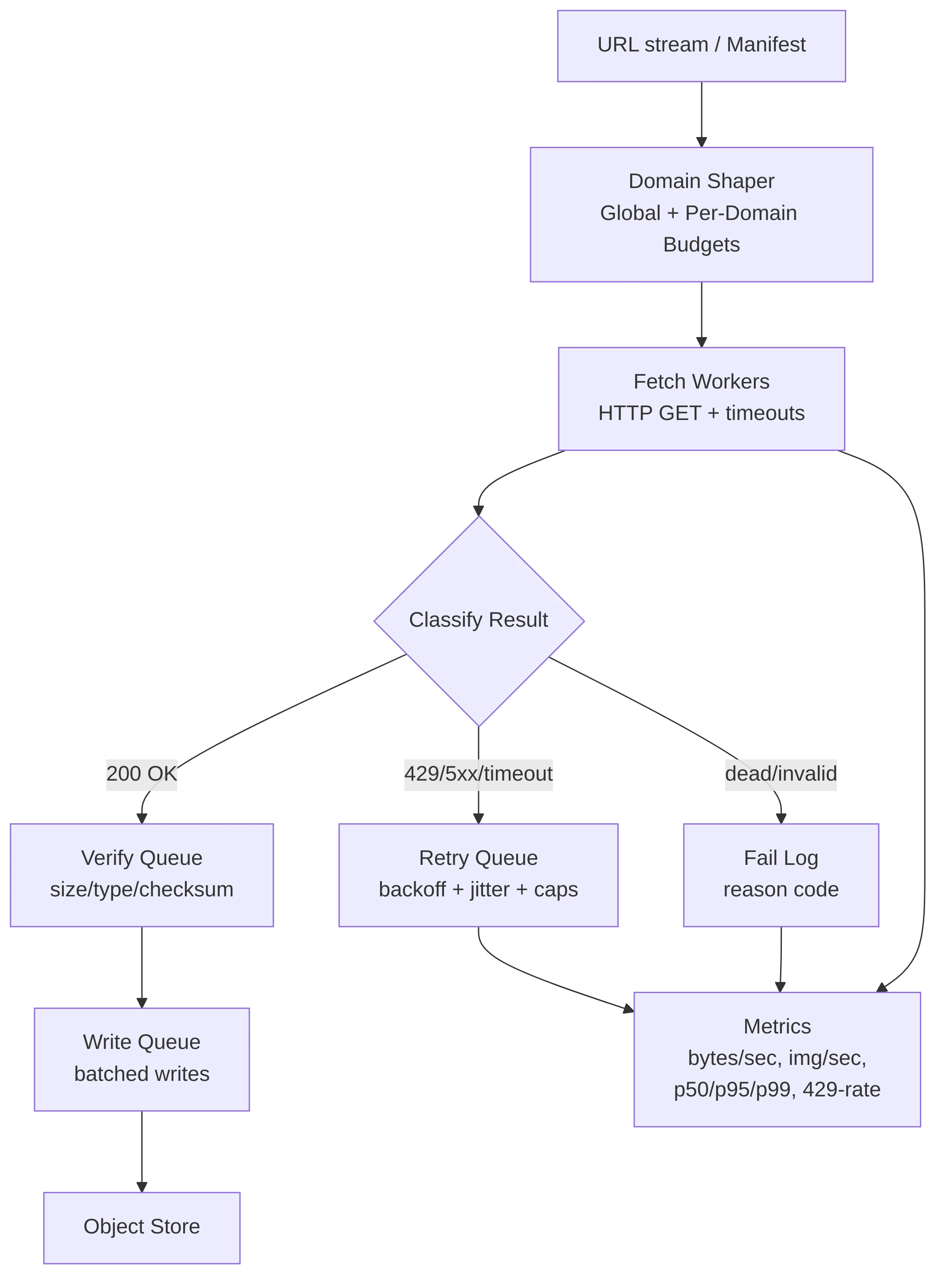
Phase 2 - Download Engine: Speed Ingestion at NIC Limits
We sustained ~1,200 images/sec across 8 H100 nodes.
Our goal was making downloads boring with stable throughput under throttling, tail latency, and internet-grade flakiness. The long pole problem moved from “waiting on bytes” to “improving data quality”.
Reality at scale (why averages lie)
At billion-scale, the taxes dominated:
-
HTTP throttling and 429 storms.
-
DNS flakiness (resolver saturation, pathological caching, transient SERVFAIL).
-
Dead links, redirects, and content drift.
-
WAF/bot checks and inconsistent origin behavior.
-
Regional latency variance and tail amplification (p99 starts steering the throughput).
-
Retries (backoff + jitter) and circuit breaking.
-
Disk flush, checksum/verification, and queueing overhead.
Our Optimizations
We didn’t chase peak QPS. We optimized for sustained throughput with guardrails:
-
Fairness: One domain can’t starve the fleet.
-
Stability: Hard timeout budgets, bounded retries, fast failure on hopeless tails.
-
Efficiency: Aggressive connection reuse to avoid handshake and DNS churn.
-
Integrity: Verify writes and metadata so ingestion doesn’t “silently succeed.”
Why Go (and why not Python)
Python could do high-concurrency I/O, and we used it for orchestration and a correctness-first reference implementation.
For the hot path, we chose Go because it provided low-overhead concurrency, predictable memory under sustained load, and a transport layer that was easy to tune and reason about when p99 behavior matters. Go’s Transport exposed knobs like MaxConnsPerHost and IdleConnTimeout explicitly, and the implementation was transparent in the standard library sources.
| Knob / Policy | What breaks without it | What we did |
|---|---|---|
| Global concurrency cap | Fleet-wide retry storms; Self-inflicted queue collapse | Hard cap across the cluster maxConcurrentDownloads = 5000; Backpressure instead of “more workers” |
| Per-domain concurrency cap | Single origin dominates; Noisy neighbor failure | Per-domain shaping + fair scheduling |
| Connection reuse (keep-alive) | CPU burn on handshakes; Ephemeral port churn; TIME_WAIT pileups | Reuse aggressively; Avoid creating new connections unless forced. MaxIdleConnsPerHost = 1000, MaxIdleConns = 5000, KeepAlive = 30s |
| Idle connection budget | Handshake churn under bursty workloads | Keep enough idle capacity to absorb bursts without reconnecting. IdleConnTimeout = 90s |
| Timeout budgets (dial/TLS/headers/body) | Tail amplification; Hung sockets pin workers forever | Explicit stage timeouts; Strict request deadline. net.Dialer.Timeout = 10s, http.Client.Timeout = 30s |
| Redirect policy | Loops; Cross-origin surprises; Wasted bandwidth | Cap redirects; Record final URL; Treat suspicious chains as failures |
| Retry budget + jitter | Thundering herd; Synchronized retries | Bounded retries; Exponential backoff with jitter; Retry caps per error class |
| 429 handling | “Retry storms” that make throttling worse | Honor Retry-After when present; Slow the domain token bucket |
| Error taxonomy | Same reaction for 429 vs 5xx vs DNS vs timeout | Different action per class: Backoff, Circuit-open, or drop |
| Write-path isolation | Disk stalls backpressure network; Throughput cliff | Separate queues for fetch vs verify vs write; Batch writes where possible. MAX_FILES_PER_DIR = 200000 |
| Verification (checksum/size/type) | Silent corruption; Poisoned dataset | Verify at ingest; Quarantine anomalies with reason codes |
We split the pipeline by the resource it stressed (Network, CPU, Disk), then enforced budgets at the edges to prevent cascading failures.
Phase 3 - Cleaning & Validation: Turning Data Into Dataset
If your metadata is wrong or your images are corrupted, you train the model to learn wrong things confidently. We enforced strict contracts at every stage: clear input/output specs per tier, logged reject reasons, and the ability to re-queue only the failed stage. This prevented the costly "reprocess everything" pitfalls.
We built a pipeline to run cheap filters first (on CPU), reject the obvious garbage, and spend expensive GPU compute only on images that survived triage. Early rejection was brutal, yet necessary.
The 10 validations
Tier 1: Decode & sanity (CPU light)
-
Decode validity: Could we parse and decode the image cleanly (JPEG/PNG/WebP)?
-
Dimensions sanity: Are width and height non-zero and within reasonable bounds for training?
[256,256] <= (W,H) <= [8096,8096]. -
Aspect ratio bounds: Are pathological panoramas and near-line images rejected? (
100:1ratio banners, ultra-tall graphics). -
Payload sanity: Did the file size matches the dimensions? (detect extreme compression. E.g.
1024×768image in10 KBsignals over-compression). We also compared content-type header against magic bytes to catch mislabeled files or CDN error placeholders.
Rejection rate at tier 1: ~2% cumulative
Tier 2: Metadata & duplicates (CPU heavy)
-
Perceptual de-duplication (pHash, Hamming distance < 5): We computed a 64-bit perceptual hash per image and identified near-duplicates. Here, one image from each cluster survived. We removed identical or near-identical variants from remixes, reposts, and mirror sites.
-
EXIF orientation normalization: We read EXIF rotation tags and corrected rotated/flipped images at the metadata level so subsequent validators (and training) would see canonical orientation. We did not re-encode, but just recorded the correction.
-
Color histogram sanity: We flagged and removed images that were nearly monochrome (solid black, solid white, or extreme overexposure) since these added noise to training.
Rejection rate at tier 2: ~11% cumulative
Tier 3: GPU-accelerated quality
-
Safety classifier: We ran a CNN-based classifier (tuned for precision) to flag sensitive content and thresholded conservatively to avoid false positives.
-
Blur detection (Laplacian variance + FFT): We measured high-frequency content using GPU-accelerated image transforms as images with near-zero high-frequency components were out-of-focus or artificially smoothed. This also caught heavily sub-sampled downscaled images.
-
Semantic alignment via embeddings: We ran CLIP-style embeddings to catch "caption says X but image is Y" misalignments. We used this as a soft filter for dataset curation, not hard removal.
Rejection rate at tier 3: ~2% cumulative
Architecture: early rejection + early feedback
We orchestrated this pipeline using Dask (dynamic task scheduler) and NVIDIA DALI (GPU image pipelines). Dask let us re-queue individual tier failures without replay. DALI's GPU-accelerated decode and transforms pushed per-node throughput from single-threaded ~1k images/sec to batched ~4k images/sec, making GPU bottlenecks the actual lever instead of I/O.
Metadata cleaning is not optional
Mismatches in metadata were silent killers. We enforced:
- No missing core fields (
dimensions,source_id,media_path,SHA) - That dimension metadata matched the decoded image (EXIF rotation-corrected).
- URL normalization and redirect resolution so re-downloads are deterministic.
- Source attribution guarantees so failed batches can be traced and removed.
By the end, we had images that were all valid, correctly oriented, deduplicated, aligned with metadata, and within the quality bounds.
Phase 4 - Quality Scoring + Tiering: Dataset Curation
Not all images taught the model equally. For instance, a sharp, well-lit photograph with strong composition and good color balance provided clear training signal while a blurry snapshot or an over-compressed graphic added noise. We scored every eligible real image and ranked the broader corpus to control what the model learned and when, turning quality into a training knob.
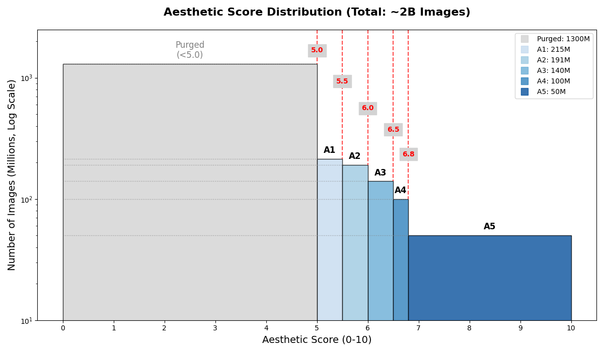
We began with ~2B downloaded images (after Phase 3), spanning both real and synthetic imagery. We ran aesthetic scoring only on the real-image subset. After filtering, this retained ~580M real images above our quality floor 5.0. We then combined them with ~115M synthetic images routed through non-aesthetic quality heuristics, yielding a final tiered corpus of ~700M images. We then organized the full corpus into five quality tiers using combined heuristics such as aesthetic score, caption lengths, caption quality and related metadata signals. These tiers gave us a curriculum lever. Early episodes sampled broadly from lower and mid quality bands to preserve diversity; later training shifted toward higher-quality subsets to sharpen composition, caption grounding, and visual detail.
The Aesthetic Predictor: SigLIP
We built a SigLIP-based image encoder + a lightweight head to predict a single scalar aesthetic_score for real images, trained on human-rated datasets (AVA-style) and internal labels. SigLIP treated each image-text pair independently via binary classification, rather than requiring batch-wide contrastive comparisons. This independence made SigLIP better suited to fine-grained similarity tasks and aesthetic assessment.
Operationally, we ran the scorer as a batched GPU inference job on 8×H100, batch size 128 and achieved a throughput of ~600 images/sec. The key design choice was making this offline and in-place: score once, persist forever and never rescore unless the scorer changed. Synthetic images bypassed this scorer and were tiered downstream using non-aesthetic signals. The counts below refer to the full tiered corpus (real + synthetic).
| Tier | Primary tier / rule | Count | Share (%) | Typical profile |
|---|---|---|---|---|
| A1 | Lowest retained quality tier | 215M | 31% | Acceptable low pass, marginal clarity or sparse captions |
| A2 | Broad mixed-quality tier | 191M | 27% | Diverse coverage, mixed composition and caption richness |
| A3 | Solid quality tier | 140M | 20% | Good composition, clearer subjects, stronger captions |
| A4 | High-quality tier | 100M | 14% | Strong visual appeal, reliable text-image grounding |
| A5 | Premium tier | 50M | 7% | Sharp, balanced, semantically rich, high-confidence supervision |
For real images, aesthetic score was one important input into tiering. For synthetic images, tiers were assigned using other quality signals such as caption quality, caption length, and related heuristics.
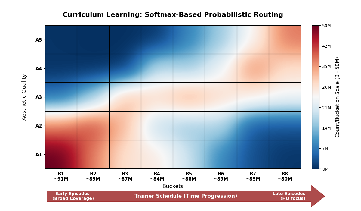
Phase 5 - Persist + Episodic Bucketing
The dataset wasn't merely “stored.” It was packaged for training dynamics.
We persisted the curated corpus with two orthogonal axes:
- 5 quality buckets (A1-A5).
- 8 episodic buckets (B1-B8).
The structure was compute-aware by design: “just keep the top tier” became suboptimal as we trained longer, because a small high-quality pool loses utility under repetition and we eventually needed broader coverage to keep the learning moving.
Two Axes, One Dataset
We treated A1-A5 as static quality labels derived from combined heuristics including aesthetic score where available, caption quality, caption length, and related metadata signals. We treated B1-B8 as dynamic curriculum label that controlled what the optimizer saw at different phases of training. Each training bucket was a mixture over multiple sources with different proportions per bucket, so we could change schedules without rewriting or copying the underlying corpus.
We used a distance-to-centers + temperature-softmax assignment which was conceptually the same idea as softmax gating used to route tokens to experts in Mixture-of-Experts (MoE) models. We computed a probability distribution over buckets using a temperature-scaled softmax, but materialized bucket membership deterministically at write-time so the same image consistently landed in the same bucket across reruns. We turned a weighted combination of quality tier and its size-bucket rank (from get_size_bucket()) into a single curriculum score .
where (we used ), and maps values to .
For each episodic bucket , we computed how "aligned" the image's score is with that bucket's center (spaced uniformly from to ):
where we set (tunable). Images close to received high logits; those far away received low logits.
Finally, we converted logits into a probability distribution over the 8 buckets using a temperature-scaled softmax:
where is the temperature parameter. Higher increases overlap (early training, broad coverage), lower concentrates probability mass (late training, tighter curriculum and higher-quality emphasis). We sampled to assign the image to bucket .
A simple pseudo-code to achieve this is as follows-
def assign_bucket(quality_tier, h, w, sigma=1.0, T=0.7, alpha=0.6, beta=0.4):
    q = (quality_tier - 1) / 4.0
    s = SIZE_BUCKET_ORDER[get_size_bucket(h, w)] # the size buckets -> ordinal
    s = s / SIZE_BUCKET_LEN                      # [0,1]
    z = alpha*q + beta*s

    mu = np.linspace(-1.75, 1.75, 8)             # centers for B1..B8
    logits = -((z - mu)**2) / (2 * sigma**2)
    p = softmax(logits / T)
    return 1 + stable_argmax(p, key=image_id)    # returns 1..8
Operational guarantees we ensured
Episodic bucketing gave us a curriculum mechanism without copying data, and it unlocked two production-grade properties:
- Stable regression isolation: During a run, we could say "the model got worse when we introduced B6 with more A3-like samples", because bucket semantics were consistent and interpretable.
- Reproducibility: The same image lands in the same bucket across reruns by using deterministic membership even if upstream curation changes.
We also soft-capped each episodic bucket to ~90M and enforced capacity at write-time so training never accidentally over-sampled a “too-easy to fill” subset (typically low-res, low-quality).
Phase 6 - Caption Curation at Billion Scale
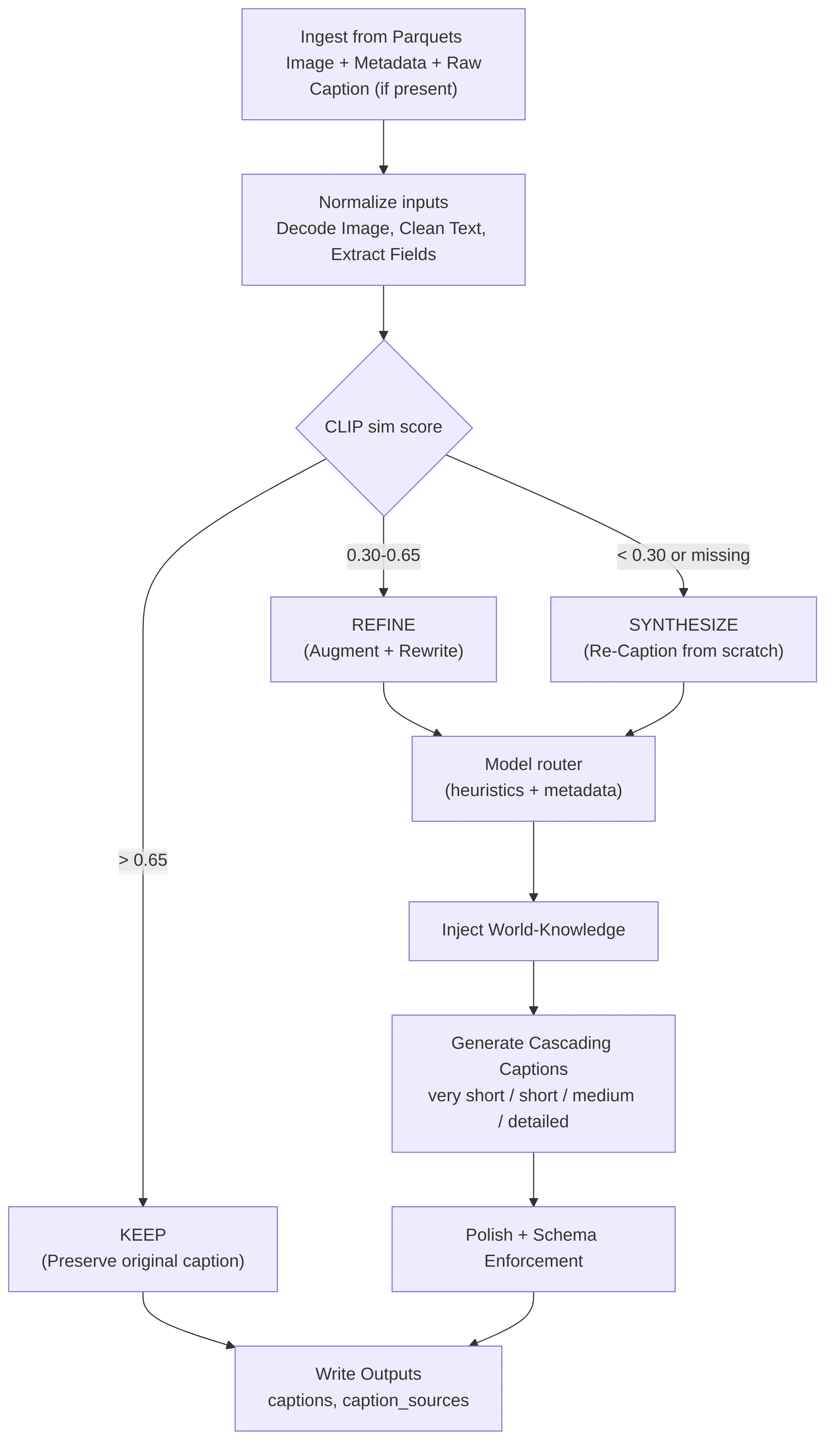
The naive approach to caption quality is discarding bad ones. At this scale, discarding bad captions would waste diversity and throw away supervision. Instead, we treated captioning as a routing and synthesis problem and not a binary keep/discard decision.
The Alignment Gate
We used CLIP's image-text similarity scoring as our routing signal because CLIP's training objective directly minimized the distance between correct image-caption pairs. Rather than a single threshold, we established a confidence-based routing table:
| Score Range | Signal | Action |
|---|---|---|
| Above 0.65 | Original captions are directionally correct | Preserve |
| 0.30-0.65 | Captions are plausible but underspecified | Refine |
| Below 0.30 | Captions are detached or missing | Synthesize |
The threshold was empirically grounded in calibration study where we validated score distributions against manual labels on a 100K-image validation slice.
The Refinement + Synthesis Pipeline: VLM Ensemble with Provenance
We ran each image cohort through a model ensemble tuned to different strengths.
| Model | Strengths | Typical Routing Criteria |
|---|---|---|
| Qwen2.5-VL | Bulk, “good-enough” captions for generic photos and web images where speed and price/throughput mattered | Default for large, untagged images and generic web imagery |
| InternVL2.5 | Used for images where hallucination risk is costly | Scientific plots, Math-heavy diagrams |
| Gemini 2.5 Flash | “Heavyweight but fast” pass for complex scenes, multi-image contexts, and long-doc images | Long PDFs (page tiles), Multi-image sets, and “hard” images |
| Claude | High-precision captions where error budget is low | Handpicked subsets, Brand assets, Legal/medical-like content, Safety-sensitive |
| LLaVA | Instruction-shaped caption generation | Routed when we needed tightly controlled styles |
| Gemma-3 | Open-source, multilingual captioner | Non-English markers, Translations for web + synthetic captions |
| InternVL3 | High-quality captioning when we wanted open-weights plus better reasoning | Used as OSS backbone images needing richer semantics |
| Qwen3 | Non-visual rewrite and fusion stage, merging VLM output with metadata | Generating multi-length variants, enforcing structure and style constraints |
| GPT‑4.1 | High Quality re-captioning + rewrite step, often conditioned on existing caption + metadata | Used during language polish + enrichment step once a factual base caption was available |
Our ground-up approach for caption refinement and re-caption pipeline:
-
Initial factual pass: We generated a seed caption using ensemble of above models based on the strengths required for the image type.
-
Metadata enrichment: We injected context from image provenance such as domain, geo-location, names, year/era info etc. to "bootstrap" world knowledge. A historical archive image becomes richer: "a person in yellow gear" became "a firefighter surveying a forest fire, ca. 1985".
-
Multi-variant generation: We produced short (1-2 sentence), medium (3-5 sentences), and long (detailed paragraph) versions.
Provenance and Metadata Tracking
We didn't erase the provenance of captions. Instead, we categorized them:
- Web Captions (20% of corpus): Passed alignment threshold unchanged.
- Web + Augmented Captions (40%): Original caption preserved; augmentation details logged.
- Synthetic Captions (40%): Fully generated; source models and scores recorded.
This granularity mapped directly to our schema: captions[], caption_sources[], caption_lengths[]. It also enabled future weighting strategies as some downstream experiments preferred "closer to human web text", while others benefited from richer synthetic descriptions.
Result: most refined images received 2–3 additional caption variants (p98: 2 captions/image), lifting the effective training corpus from ~700M images to ~1.5B image-caption pairs. Caption curation signals fed back into how we ranked and tiered the corpus, especially for synthetic images where aesthetic scores were unavailable.
The Engineering Reality: Limits and Trade-Offs
At our scale, two practical constraints dominated:
-
Compute: Computing cosine similarity between 700M images and their captions was
O(M)in naive form. We arrived at a stable throughput via distributed CLIP scoring across 32 GPUs using a batch-wise reduce approach. The pipeline phases included image decoding, batching GPU inference, I/O sharding which kept workers saturated for weeks under contention. -
Synthetic caption quality ceiling: High-performing VLMs like GPT-4.1 generated captions with quality approaching human annotations (~4.0/5 mean ratings in LAION-COCO evaluation), but weaker models introduced variance. We standardized on stronger models at the cost of throughput.
The payoff was substantial. Before Phase 6, ~80% of captions in our image dataset were misaligned or uninformative. After:
- Every image had a meaningful caption paired to it.
- Average caption length increased from ~8 words to ~50 words (depending on category).
- CLIP alignment scores for the full corpus shifted right as the long tail of near-zero alignments disappeared.
Phase 7 - Augmentation: Multiplying HQ Data Without Degradation
Even at billion scale, models plateaued during late-stage training where compositional detail and rare-but-critical concepts mattered more than breadth. Synthetic augmentation offered a way to surface new variations without collecting new images. But the trap was easy: aggressive augmentations could erode semantic fidelity and poison the entire pool.
We augmented only the top 30% quality tier. The premise was simple: low-quality images don't improve with modification. But for premium images, controlled variation is powerful.
The CLIP Similarity Constraint
But how much variation is "safe"? We employed CLIP image-embedding similarity as a guardrail. CLIP embeddings capture semantic content, so two images with cosine similarity >=0.90 were treated as semantics-preserving. We computed:
If an augmentation dropped similarity below 0.90, we discarded it. Empirically, this threshold balanced diversity gains against distribution fidelity for us.
Our Augmentation Portfolio
We applied a controlled suite of transformations:
- Rotation: +-30° (discrete steps) to prevent orientation fixation.
- Flips: horizontal to preserve semantic and spatial understanding.
- Crops & Zoom: Random crops within constrained bounds to simulate frame variation.
- JPEG Recompression (Q > 70): real-world compression noise to mirror distribution of web images.
- Color Jitter: ±5% brightness, ±10% contrast to simulate lighting variance without drastic shift.
- Grayscale: Enable monochrome robustness for ~10% of augmented images.
- Mild Noise/Grain (Gaussian, σ ≤ 2): Sensor noise tolerance.
- Downscale/Upsample Artifacts (controlled, 1–2 resampling passes): Compression/resolution variations.
We avoided perspective warping, severe crops, extreme noise, and "mosaic" (multi-image tiles). These shattered CLIP embeddings and created unnatural distributions.
Orchestration & Tail Set Gambit
- We generated augmentations online during training using NVIDIA DALI pipelines on GPUs, to avoid disk bottlenecks. A lightweight Python validator checked CLIP similarity per batch, and ensured rejected augmentations never reached training loops. This reduced rework and kept augmentation "soft" (not mandatory in every epoch).
- We added a curated "tail" of premium images (
aesthetic_score >= 7.0,clip_score >= 0.95, and long-form descriptions). This tail was not augmented. This was done to introduce more detail and composition. Pristine, semantically rich examples would prevent model collapse and force the model to refine.
Phase 8 - Upload & Storage Layout: Engineering at Scale
Pushing billion images into cloud storage wasn't a "copy operation." At this volume, every architectural decision compounded: prefix sharding, concurrency models, checksum strategies, and error recovery all collapsed into throughput. We sustained ~1,500 images/sec on a 4-VM pool.
The Core Challenge: Prefix Hot-Spotting
Google Cloud Storage (GCS) auto-scaled based on object key distribution. Without deliberate sharding, sequential uploads (especially with monotonically increasing IDs/timestamps) would create hot spots in the key index. GCS detected and rebalances these, but rebalancing took minutes.
Our strategy: Partition the dataset into 1,000 logical shards before upload, encoding the shard ID directly into the object prefix. Each image got a path like:
gs://<bucket>/images/bucket=<episodic>/aesthetic=<tier>/pk=<0-999>/id=<hash>.jpg
By distributing writes evenly across 1,000 prefixes upfront, we avoided a painful ramp-up. GCS's auto-scaling detection became irrelevant when load was already uniform.
Optimizations at Scale
- Although individual images were small (<1MB), we grouped them into ~500MB tarballs before upload. Files greater than 150MB triggered GCS's parallel composite upload mechanism, which split the file into up to 32 chunks, uploaded them in parallel, and composed them server-side. For a 500MB tarball, we achieved ~2x throughput improvement over single-threaded upload.
- With millions of objects, listing was slow and expensive for validation. Instead, we maintained manifest files, a simple record of uploaded batches with checksums. Validating completeness meant checking the manifest.
Four VMs, each running an uploader service consumed from a shared parquet metadata stream. Each VM saturated at roughly 375 images/sec, constrained by network bandwidth.
What We Learned
-
Captions were the training signal. Improving text moved quality far more than comparable effort on image filtering.
-
Single thresholds threw away value. Episodic bucketing let us run a curriculum where broader coverage was learned early and high-signals paired later without losing diversity.
-
Every stage needed a contract. Schema + Invariants + Metrics + Failure budgets, or the pipeline turned into folklore.
-
Determinism wasn’t optional. Versioned manifests + Content Hashes made any slice reproducible, which made model regressions explainable.
At billion-scale, the dataset became a model component: it encoded behavior, bias, and failure modes as directly as architecture and optimizer choices.
Appendix
For readers who want the complete end-to-end view, the diagram below shows how metadata records moved from Parquet → Kafka topics → stage-specific worker pools → until assets landed in final object storage.
References
- Engineering OSS Packages/Libraries: Apache Parquet Format, kafka-sarama, Perpetual Hashing, Google PCU, Dask
- Models that helped us: InternVL, QwenVL3, Google Gemma, Gemini2.5-Flash, LLaVA
- NVIDIA: DALI, NeMo
- Noteworthy Research: CLIP, SigLIP
Created by NucleusAI. Excited to work with us? Drop an email at contact@withnucleus.ai