mHC-Triton: Building a 6× Faster Kernel for DeepSeek's Hyper-Connections
2026-01-28
TL;DR
We present mHC-Triton, an open-source implementation of DeepSeek's Manifold-Constrained Hyper-Connections paper with fused Triton kernels that achieve:
- 6.2× faster full forward+backward vs PyTorch baseline
- 1.3× memory savings through intelligent recomputation
- 3.4× overhead vs simple residual connections (acceptable cost for richer architecture)
- FSDP2 support
This post walks through the theory, engineering decisions, and kernel optimizations that make efficient mHC training possible.
1. The Residual Bottleneck Problem
The Legacy of Identity Mapping
Since ResNet (2015) and the original Transformer (2017), deep networks have relied on the simple residual formula:
This "identity mapping" ensures gradients flow through arbitrarily deep networks without vanishing. It's elegant, simple, and has powered every major language model from GPT to LLaMA.
But there's a problem: as models scale, this single-stream path becomes a bandwidth bottleneck.
All information—from every attention head, every layer, every token—must squeeze through one vector. The residual stream becomes a crowded highway with no express lanes.
Hyper-Connections: The Promise
Researchers at ByteDance proposed "Hyper-Connections": instead of one residual stream, use multiple parallel streams that can interact and mix information. Think of it as upgrading from a single-lane road to a multi-lane highway with interchanges.
The idea is compelling:
- Richer feature reuse: Information can take different paths through the network
- Learnable topology: The network decides how layers connect
- Increased bandwidth: Multiple streams carry more information
The Stability Crisis
Here's where things get interesting. DeepSeek found that at scale (27B+ parameters), unconstrained hyper-connections are catastrophically unstable.
The problem: small amplification errors in the learnable mixing matrices compound exponentially across layers. In their experiments, signal norms exploded by >3000×, causing training to diverge completely.
This is the core insight of the mHC paper: you can't just add more streams—you need mathematical guardrails.
2. DeepSeek's mHC Solution
The Mathematical Constraint: Doubly Stochastic Matrices
DeepSeek's key innovation is constraining the mixing matrices to the Birkhoff Polytope—the set of all doubly stochastic matrices where every row and column sums to exactly 1.
Why does this work? A doubly stochastic matrix is like a "probability redistribution" operator:
- It can shuffle information between streams
- But it cannot amplify the total signal magnitude
- The constraint is differentiable and learnable
 The Sinkhorn-Knopp algorithm converges to a doubly stochastic matrix by alternating row and column normalization.
The Three Core Operations
The mHC layer implements three operations:
Pre-mixing (weighted combination of streams):
Residual mixing (doubly stochastic transform):
Post-distribution (route output back to streams):
Where:
- — normalized weights for combining streams into layer input
- — doubly stochastic 4×4 matrix (via Sinkhorn-Knopp)
- — distribution weights for routing output back
Dynamic Weights
The mixing weights aren't static—they're computed from the input via a learned projection:
This makes the architecture input-dependent: different inputs can take different paths through the network.
3. Engineering the Triton Kernels
Here's where the real work begins. The mathematical framework is elegant, but naive implementation is unacceptably slow.
The Memory Wall Problem
With 4 parallel streams, you have:
- 4× more activations to store
- 4× more memory traffic
- Multiple small operations that are bandwidth-bound
A naive PyTorch implementation launches many small kernels, each reading from and writing to global memory. The GPU spends more time moving data than computing.
Optimization 1: Aggressive Kernel Fusion
Key insight: fuse everything possible into single kernel launches.
 Left: Multiple kernel launches with memory round-trips. Right: Single fused kernel.
The _fused_dynamic_weights_kernel computes all these steps in one pass:
# Single kernel does ALL of this:
# 1. Mean pooling
# 2. Matrix multiplication (x @ φ)
# 3. RMS normalization
# 4. Scaling and bias
# 5. Sigmoid activations
# 6. Softmax normalization for H_pre
# 7. Full Sinkhorn-Knopp iteration for H_res

@triton.jit
def _fused_dynamic_weights_kernel(
    x_ptr, phi_t_ptr, bias_ptr,
    alpha_pre, alpha_post, alpha_res,
    H_pre_ptr, H_post_ptr, H_res_ptr,
    batch, in_dim,
    BLOCK_K: tl.constexpr,
    sinkhorn_iters: tl.constexpr,
    eps: tl.constexpr,
):
    # ... 400 lines of fused operations
Result: 7.9× speedup on dynamic weight computation alone.
Optimization 2: Register-Based 4×4 Matrices
A 4×4 matrix has only 16 elements. This fits perfectly in GPU registers!
 16 scalar registers hold the entire matrix—no shared memory needed.
# Load 4x4 matrix to registers
m00 = tl.load(M_ptr + base + 0)
m01 = tl.load(M_ptr + base + 1)
# ... all 16 elements

# Row normalization entirely in registers
r0 = m00 + m01 + m02 + m03 + eps
m00 /= r0; m01 /= r0; m02 /= r0; m03 /= r0
This approach:
- Eliminates shared memory bank conflicts
- Maximizes instruction-level parallelism
- Keeps the entire Sinkhorn computation in registers
Optimization 3: Transposed Weight Matrix Layout
The projection matrix φ has shape [in_dim, 24] where in_dim = 4 × hidden_dim (e.g., 16,384 for dim=4096).
Naive layout problem: Reading column vectors from a row-major matrix causes strided memory access—the worst pattern for GPU bandwidth.
Solution: Store φ transposed as [24, in_dim]. Now each output dimension's weights are contiguous:
# COALESCED: Each row read is contiguous in memory
phi0 = tl.load(phi_t_ptr + 0 * in_dim + k_offs, mask=k_mask)
phi1 = tl.load(phi_t_ptr + 1 * in_dim + k_offs, mask=k_mask)
# ... 24 coalesced reads
Optimization 4: O(T²) Recomputation for O(1) Memory
The Sinkhorn-Knopp algorithm runs T iterations (typically T=20). A naive backward pass would store all T intermediate matrices—that's 20× memory overhead.
 Left: Store all intermediates. Right: Recompute on demand.
Approach: store only the original input, recompute forward states during backward.
# Backward: for each iteration, recompute forward states
for _iter in range(num_iters):
    target_iter = num_iters - 1 - _iter

    # Recompute forward from M_orig to target_iter
    m = abs(M_orig) + eps
    for _fwd in range(target_iter):
        # row/column normalization
        ...

    # Now compute backward through this iteration
    ...
Trade-off: O(T²) compute for O(1) memory. For T=20 with tiny 4×4 matrices, this is 20× memory savings at negligible compute cost.
Optimization 5: Hybrid Gradient Reduction
Weight gradients require summing over (batch, seq, dim) axes. We use a two-phase approach:
- Triton kernel: Compute partial sums per
(batch, seq, dim_block)tile - PyTorch: Final reduction using highly-optimized
tensor.sum()
# Triton: partial sums per tile
dH_post_partial = torch.empty(batch, seq, num_d_blocks, 4, ...)

# In kernel: write partial sums
tl.store(partial_base + 0, tl.sum(tl.where(d_mask, dh0 * branch, 0.0)))

# PyTorch: final optimized reduction
dH_post = dH_post_partial.sum(dim=(1, 2))
This hybrid approach beats both pure-Triton and pure-PyTorch alternatives.
4. Benchmarks & Results
All benchmarks run on NVIDIA H100 80GB HBM3 with batch=16, seq=2048, dim=4096.
Speed Comparison

| Operation | PyTorch | Triton | Speedup |
|---|---|---|---|
| Sinkhorn (20 iter) | 0.74ms | 0.47ms | 1.6× |
| Stream Mix | 8.53ms | 1.00ms | 8.6× |
| Add Residual | 2.57ms | 0.89ms | 2.9× |
| Dynamic Weights | 0.90ms | 0.11ms | 7.9× |
| Full Forward+Backward | 85.00ms | 13.66ms | 6.2× |
The stream mixing kernel shows the largest speedup (8.6×) because it benefits most from fusion—the PyTorch version requires multiple einsum operations with intermediate tensors.
Memory Comparison

| Operation | PyTorch | Triton | Savings |
|---|---|---|---|
| Sinkhorn Backward | 120.0MB | 68.0MB | 1.8× |
| Full Forward+Backward | 8003.6MB | 6162.8MB | 1.3× |
The recomputation strategy provides 1.8× memory savings on Sinkhorn alone. Combined savings across the full pass are 1.3×.
Residual Stream Gain Analysis
A key validation of mHC's stability: the composite amax gain magnitudes of the residual streams remain bounded during training. The doubly stochastic constraint prevents the exponential amplification that plagued unconstrained hyper-connections.
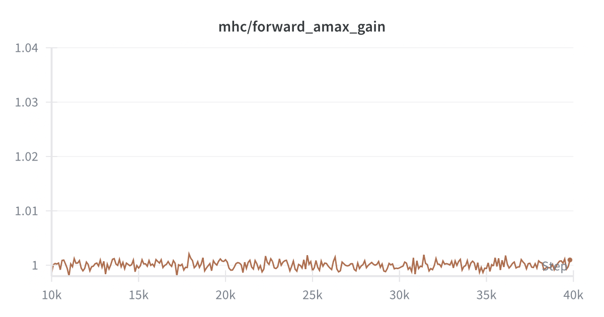 Composite forward gain across all layers.
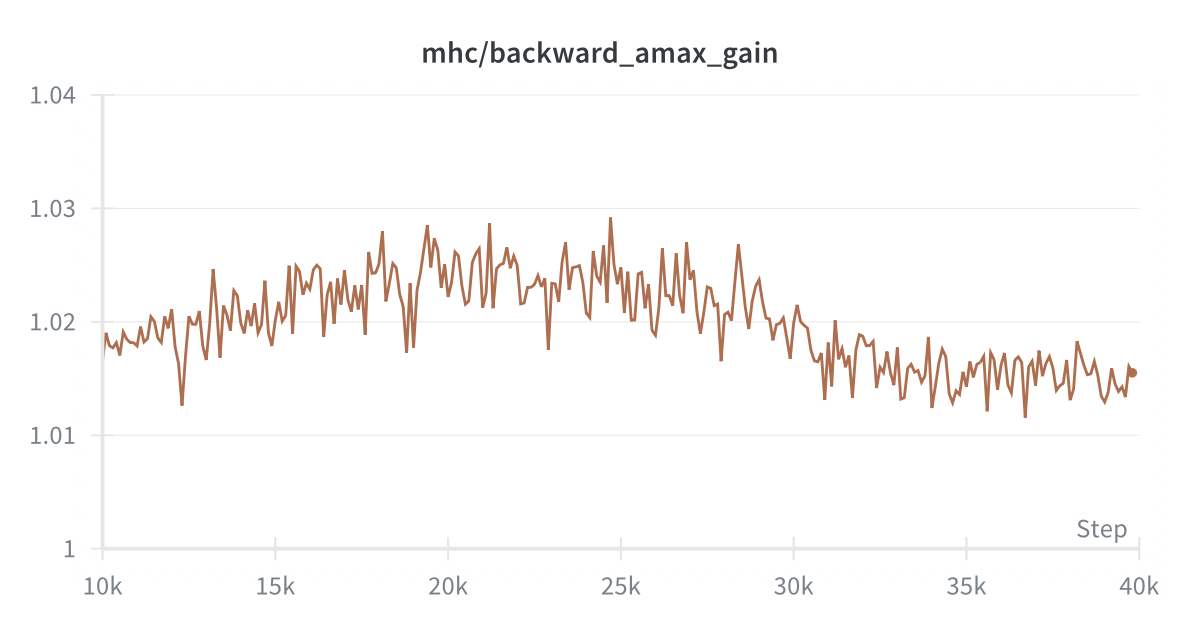 Composite backward gain across all layers.
These visualizations confirm that both forward and backward passes maintain stable gain magnitudes across layers—a direct result of the Birkhoff polytope constraint.
5. Usage Guide
Installation
pip install git+https://github.com/NucleusAI/mHC-triton.git
Quick Start
import torch
from mhc import HyperConnection

# Create hyper-connection layer
hc = HyperConnection(
    dim=512,           # Hidden dimension
    num_streams=4,     # Parallel streams (must be 4)
    dynamic=True,      # Input-dependent weights
    sinkhorn_iters=20, # Iterations for doubly stochastic projection
).cuda()

# Input: hyper-hidden state (batch, seq, num_streams, dim)
H = torch.randn(2, 128, 4, 512, device='cuda')

# Forward pass
branch_input, add_residual, H_res = hc(H)

# Your layer (attention, MLP, etc.)
branch_output = my_transformer_layer(branch_input)

# Combine with residual streams
H_new = add_residual(branch_output)
Architecture Overview

The flow is:
- H (hyper-hidden) enters the module
- Dynamic weights computed from mean-pooled H
- Stream mix produces branch_input for your layer
- Your layer processes branch_input → branch_output
- Add residual combines branch_output with H_residual → H_new
Integration with Existing Models
To replace standard residuals with HyperConnection:
# Before (standard residual)
class TransformerBlock(nn.Module):
    def forward(self, x):
        x = x + self.attention(self.norm1(x))
        x = x + self.mlp(self.norm2(x))
        return x

# After (with HyperConnection)
class HyperTransformerBlock(nn.Module):
    def __init__(self, dim):
        self.hc_attn = HyperConnection(dim, layer_idx=0)
        self.hc_mlp = HyperConnection(dim, layer_idx=1)
        # ... attention, mlp, norms

    def forward(self, H):  # H: [batch, seq, 4, dim]
        # Attention block
        branch_in, add_res, _ = self.hc_attn(H)
        H = add_res(self.attention(self.norm1(branch_in)))

        # MLP block
        branch_in, add_res, _ = self.hc_mlp(H)
        H = add_res(self.mlp(self.norm2(branch_in)))

        return H
Low-Level API
For researchers who want fine-grained control:
from mhc import (
    sinkhorn_knopp,
    fused_stream_mix,
    fused_add_residual,
    fused_dynamic_weights,
)

# Project any matrix to doubly stochastic
M = torch.randn(batch, 4, 4, device='cuda')
P = sinkhorn_knopp(M, num_iters=20)  # P.sum(dim=-1) ≈ P.sum(dim=-2) ≈ 1

# Stream mixing
branch_input, H_residual = fused_stream_mix(H, H_pre, H_res)

# Residual addition
H_new = fused_add_residual(H_residual, branch_output, H_post)

# Dynamic weight computation
H_pre, H_post, H_res = fused_dynamic_weights(
    x, phi, bias, alpha_pre, alpha_post, alpha_res
)
FSDP / Distributed Training
The module is designed for distributed training compatibility:
# Scalar parameters are 1D tensors with numel==1 for FSDP compatibility
self.alpha_pre = nn.Parameter(torch.tensor([init_scale]))
self.alpha_post = nn.Parameter(torch.tensor([init_scale]))
self.alpha_res = nn.Parameter(torch.tensor([init_scale]))
6. Conclusion
What We Learned
Building mHC-Triton taught us several lessons about GPU kernel engineering:
-
Kernel fusion is essential for memory-bound operations. The 6.2× speedup comes primarily from eliminating memory round-trips.
-
Small matrices are register-friendly. The 4×4 constraint isn't just a limitation—it's an optimization opportunity. 16 registers per matrix enables fully in-register computation.
-
Recomputation beats storage for iterative algorithms. Trading O(T²) compute for O(1) memory is excellent when T is small and matrices are tiny.
-
Hybrid approaches work. Using Triton for the compute-intensive parts and PyTorch for reductions leverages the best of both worlds.
The Bigger Picture
mHC represents a shift toward learnable architecture. Instead of hard-coding how layers connect (single residual stream), we're learning the optimal topology.
This has profound implications:
- Different inputs can take different paths
- The network can specialize streams for different features
- Training dynamics may be fundamentally different
Future Directions
- Variable stream counts: Current implementation requires exactly 4 streams. Generalizing to N streams would enable architecture search.
- FlashAttention integration: Fusing mHC with memory-efficient attention could further reduce overhead.
- Quantization: INT8/FP8 kernels for inference optimization.
Try It Yourself
pip install git+https://github.com/NucleusAI/mHC-triton.git
The code is open source. We welcome contributions, bug reports, and discussions!
References
- Hyper-Connections (DeepSeek, arXiv:2512.24880)
- Triton: An Intermediate Language and Compiler for Tiled Neural Network Computations
- Sinkhorn-Knopp Algorithm
Created by NucleusAI. If you found this useful, please star the repo!